Sparse Bills, Better Forecasts

John Rula, PhD — Chief Technology Officer

If you’ve ever tried to build an energy baseline from 5 months of utility bills, you know the pain. Standard change-point models fall apart — sometimes spectacularly. This post is about why, how bad the problem actually is, and what we built at Energy Pilot AI to handle it differently.

In our work with retrofit sellers, A&E firms and ESCOs, we see the same problem again and again. A prospective customer hands over twelve months of utility bills — if you’re lucky. More often it’s eight months. Or five. Or a handful of PDFs with inconsistent billing periods and a gap where someone changed accounts.

From this, you’re expected to build a credible energy baseline, estimate savings for a proposed retrofit, and produce numbers that will survive M&V scrutiny. The tools most of us reach for — change-point regression, degree-day models, LEAN analysis — were designed for a world where you had clean, complete data. They work well enough when you have it. When you don’t, they break in ways that are hard to see and expensive to discover later.

At NZero, we’ve used our years of experience in energy data analysis and forecasting to try and alleviate this common bottleneck and pain point: this post is about what we’ve learned, why the sparse-data problem is more consequential than most people realize, and a new forecasting approach we’ve built at Energy Pilot AI that handles it differently.

The hidden cost of incomplete billing data

The standard industry approach to utility bill forecasting follows a well-worn path. Collect monthly billing data. Regress energy consumption against heating and cooling degree days. Fit a change-point model — maybe a 3-parameter cooling model, maybe a 5-parameter model if the building has both heating and cooling loads. Use the model to normalize consumption to a typical meteorological year. Produce a baseline.

This works well, and is a trusted and proven process, and it aligns with ASHRAE and IPMVP requirements. But the approach carries an implicit assumption: you have enough data to fit the model reliably. A 5-parameter change-point model needs to identify two balance points and three slopes. With twelve clean monthly observations, that’s twelve data points to estimate five parameters. With seven months of data, especially if they cluster in one season, you’re asking the model to extrapolate through regions of the degree-day space it has never seen.

This isn’t a theoretical concern. In our experience, the typical sales engagement starts with partial data:

• Utility bill PDFs that cover 3–6 months, not 12
• Billing periods that don’t align with calendar months
• Gas accounts that were opened or closed mid-year
• Portfolio assessments where some buildings have years of data and others have almost none

If you’re screening retrofit opportunities and your prospect can only provide a few months of bills, this is the gap we’re closing. The sparse-data problem doesn’t just affect model accuracy — it determines whether your team can qualify a deal at all.

The problem with regression models is that they are not just trained only on what’s known, but also evaluated only against that same given set. When you fit a regression model to sparse data, it converges to what’s there — the R² might even look reasonable — however it’s missing a large part of the picture. This is especially true when single seasons are represented. Using summer behavior to predict winter usage is challenging at best.

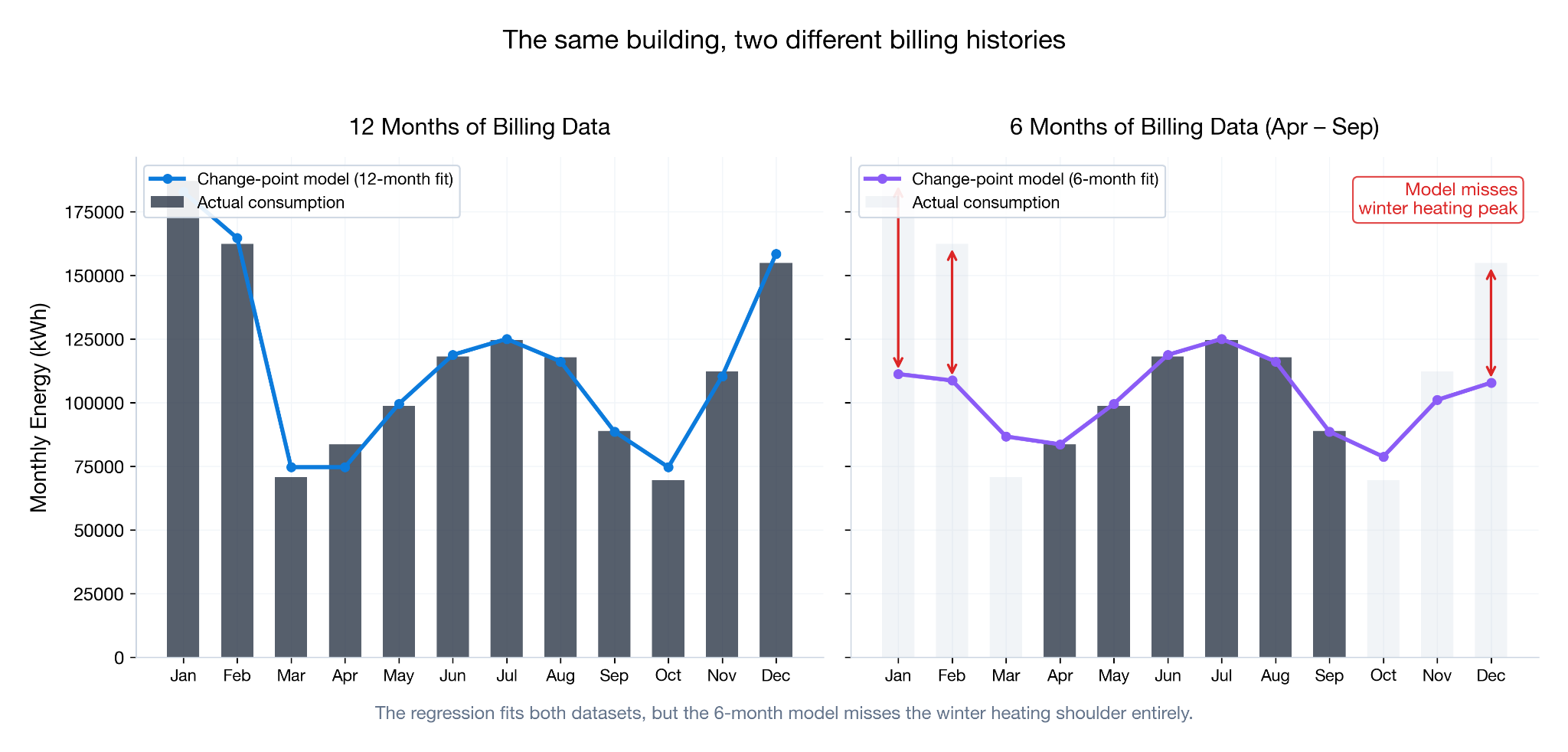
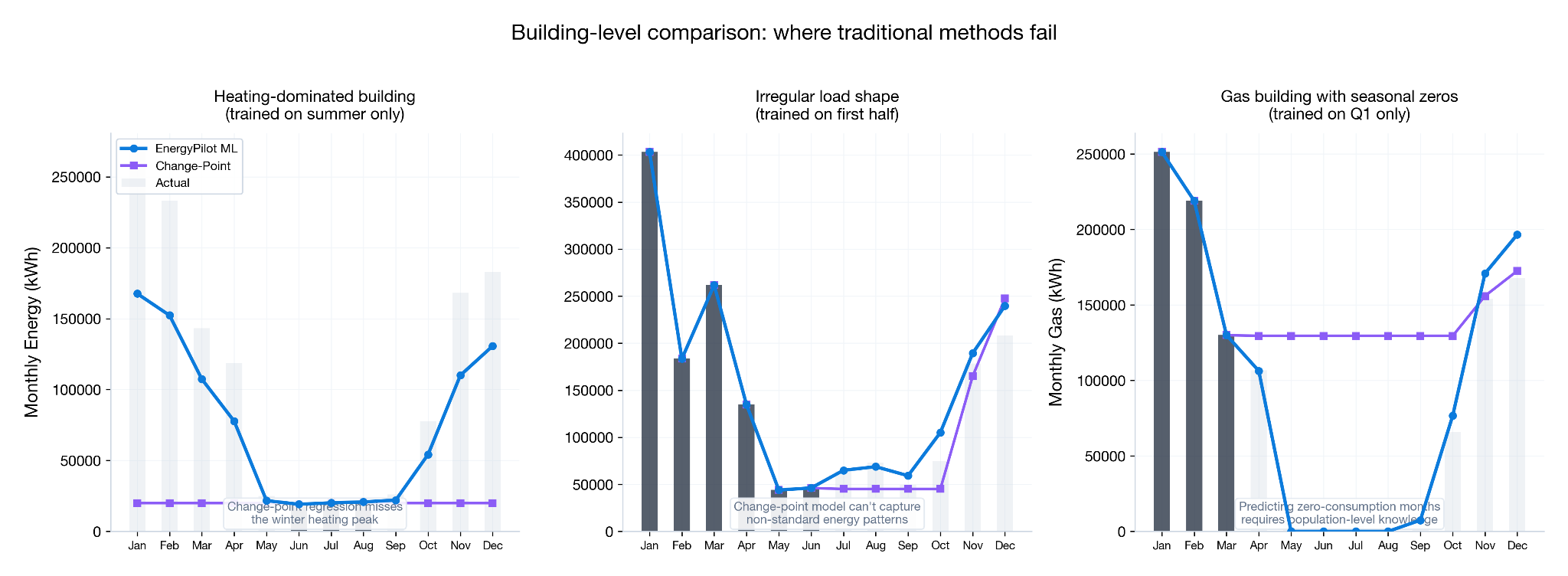
The figure below illustrates this effect: with 12 months of utility data, the 5-parameter change point model closely tracks with the measured data, yet with 6 months of summer billing data the model grossly undershoots winter utility usage. Without the context of heating behavior, the model performs poorly in isolation — it is unable to know how this particular building behaves, and cannot pull from a population of similar buildings.

This is a real problem in the early-stage screening of retrofit opportunities. If your baseline is off by 15% on a 50,000-square-foot building, your savings estimate is off by a proportional amount, and significantly impact your qualification decisions: you may be pursuing — or passing on — projects based on unreliable numbers. This is the gap Energy Pilot AI is designed to fill.

A different starting point: what if the model already knew something about your building?

The approach we’ve developed for Energy Pilot AI starts from a different premise. Instead of treating each building as a blank slate, we start with a model that already understands how commercial buildings use energy — trained on hundreds of thousands of building energy profiles spanning every major building type, climate zone, vintage, and fuel type (in the US).

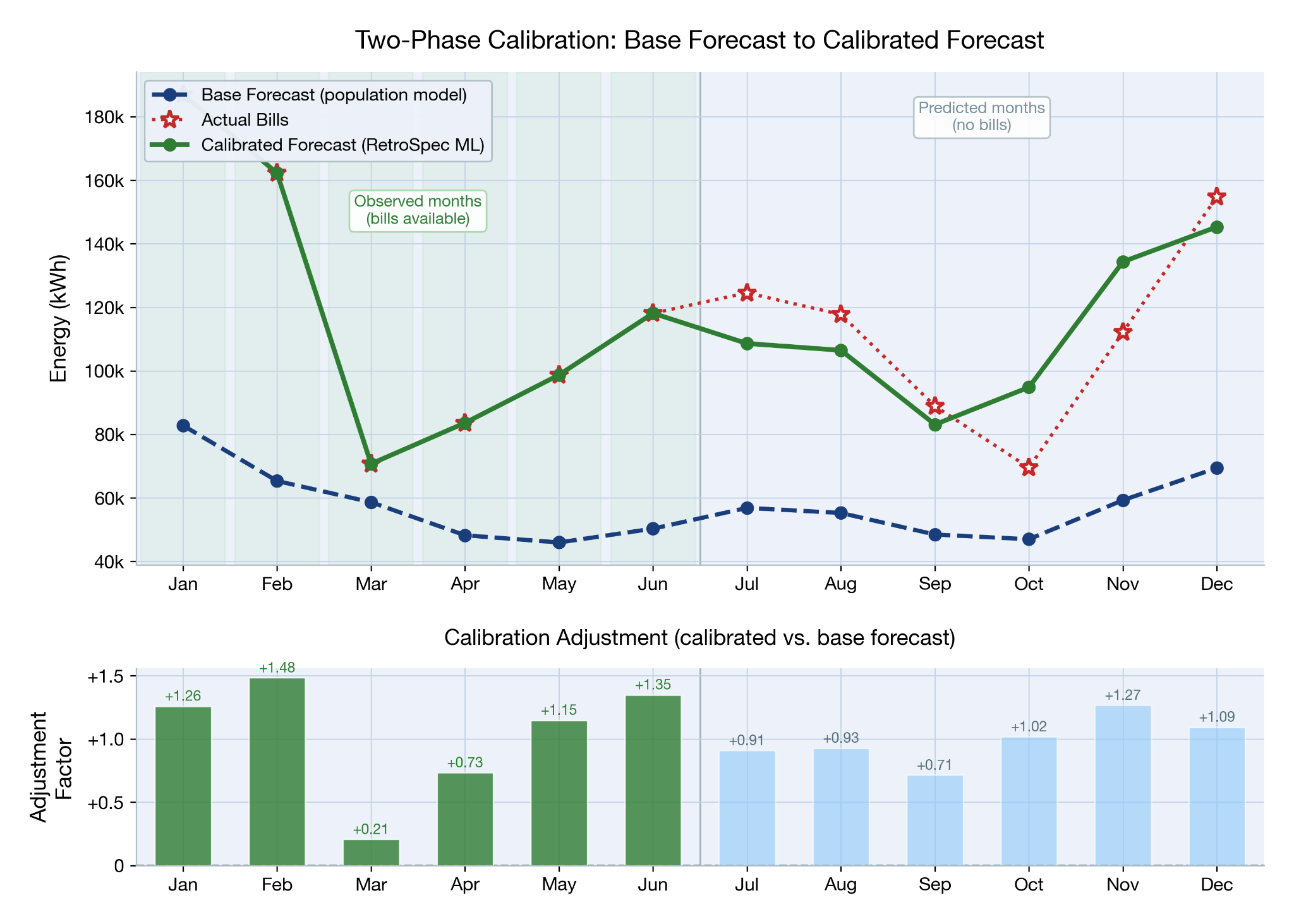
This base model acts as a strong prior. Given a building’s metadata — type, size, location, age, HVAC system — it produces a twelve-month energy consumption profile that reflects what a building like yours typically uses. Not perfectly. Not for your specific building. But a well-informed starting point that captures the broad seasonal shape, the scale, and the climate response. This is shown as the blue dashed line in the figure below.

Then, when actual utility bills arrive, a second model takes over. This calibration model compares the base prediction to real billing data for the months you have, learns how your building specifically deviates from the population pattern, and applies building-specific corrections to every month — including the ones you haven’t observed. The adjustment factors below show what is fed into the calibration model (green bars) and the adjustment factors output for the remaining months (blue bars).

The key insight is that the calibration model doesn’t just compute a simple scaling factor. It learns structured corrections: your building’s winter bias might be different from its summer bias. The confidence of the correction depends on how many months of evidence you’ve provided and how close those months are (seasonally) to the month being predicted. And it produces calibrated uncertainty bounds — wider when the evidence is thin, narrower when it’s strong.

In Energy Pilot AI, this all occurs through a simple workflow within the application. Energy data is imported, either through CSV uploads, automated PDF bill OCR, or manual entry. Once in the system, the platform’s forecasting models work seamlessly from existing energy data and any known building information — such as existing HVAC systems — to forecast calibrated energy load for the missing months.

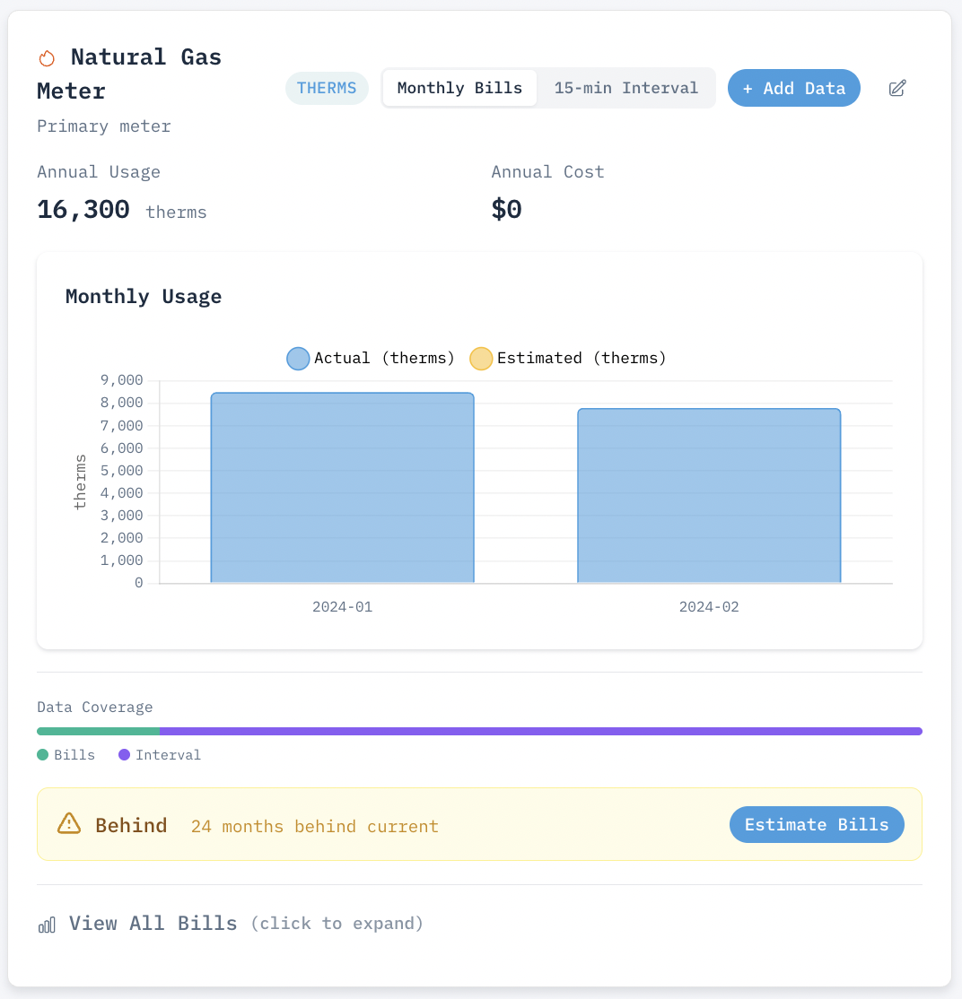
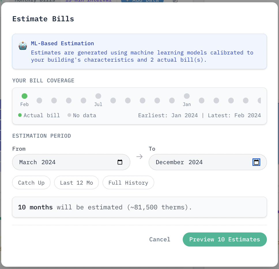
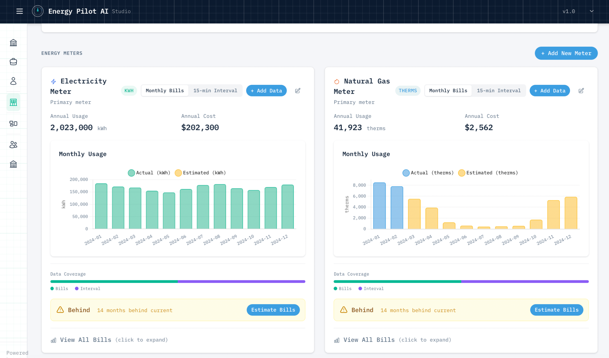
As seen in the images above, using only 2 existing natural gas bills from winter, we can easily estimate the remaining 10 months of the year, including summer months with little usage.

How it performs

We evaluated our two-phase machine learning approach against two standard methods, and a calibrated population approach, testing across a large test set of buildings with known complete consumption data. We utilized NREL’s ComStock End-User Load Profiles (EULP) for our evaluation, to provide a diverse set of building models with 12 months of complete energy usage.

5-Parameter Change-Point Model: Common change-point model for ASHRAE, two modeled change-points modeling baseload, heating and cooling sensitivities. This is the industry standard for utility data estimation and prediction.

Degree-Day Regression: Three parameter regression models correlated to observed heating and cooling degree days, and is still common across the industry for a slightly simplified approach compared to the change-point models above.

Naive Population Calibration: A custom strawman approach we developed for evaluation, using the same population usage data as our training data, and calibrated/scaled through the ratio of observed energy compared to the population mean for each month. We created this to understand how much the machine learning model contributes to improvements compared to population priors and simple ratio scaling.

The evaluation simulated realistic data availability scenarios: for each building, we withheld a random subset of months and asked each method to predict the missing months using only the remaining observations.

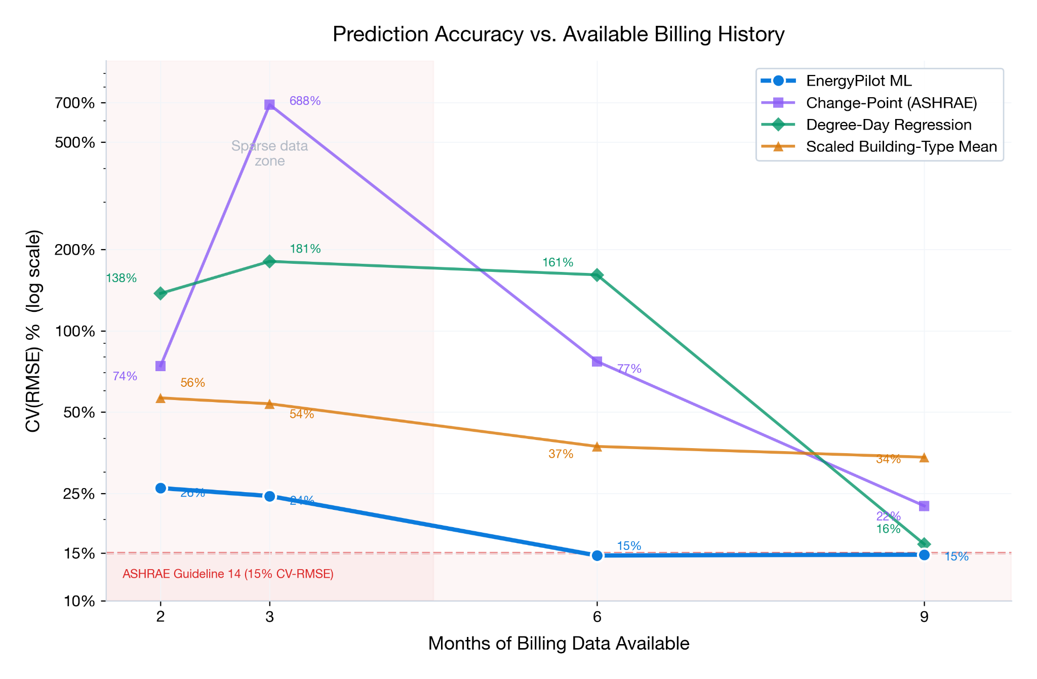
Change-point model accuracy degrades sharply with fewer months of billing data. Below 8 months, 5-parameter models become unreliable for annual estimates. The 3-month spike for change-point models is indicative of the split season training, where winter bills are used to predict summer months, and vice versa.

Two findings stood out:

At 9+ months of data, all methods perform reasonably well. This is expected — with near-complete data, even simple regression has enough to work with. Our approach still showed improvements, but the gap was modest.

Below 6–7 months, the gap becomes significant. This is where traditional regression starts extrapolating into unseen conditions, and where our population-informed calibration approach provides its largest advantage. At 3 months of available data, our method’s median prediction error was 24.4% compared to 688% for 5-parameter change-point regression.

What this means for the retrofit industry

We built Energy Pilot AI to solve a practical problem: the early-stage screening of retrofit opportunities takes too long and produces unreliable numbers when data is incomplete. ESCOs, engineering firms, and equipment manufacturers all face this. The technical audit gets the detailed analysis right — and we have approaches to assist here too — but by the time you’re doing a technical audit, you’ve already invested significant resources in pursuing the project. The question is whether the projects you’re pursuing are the right ones.

Better baselining through utility bill forecasting — especially when billing data is sparse — makes early-stage screening faster and more reliable. It means:

Larger funnel, better qualification. You can screen more buildings with less data, which means you can evaluate portfolio opportunities that would be impractical to assess building-by-building with traditional methods. Complete utility data is no longer a bottleneck for deal flow.

Faster speed to proposal. When you don’t need twelve clean months of billing data to produce a credible baseline, the time from first contact to preliminary savings estimate shrinks considerably.

We’ll be sharing more about Energy Pilot AI’s capabilities in the coming months — including how we handle portfolio-scale analysis, retrofit measure modeling, and integration with existing M&V workflows. If you work in the retrofit space and deal with the challenges we’ve described here, we’d like to hear from you.